A great systematic review by Schwarze et.al. in Genetics in Medicine on the cost benefits of Whole Genome Sequencing (WGS) and Whole Exome Sequencing (WES) in the clinical settings.
Main findings that interested me:
Doing molecular testing (using single-gene, panel testing, or microarrays) for genetic disorders only results in 50% molecular diagnosis. Many patients will still be going on extensive diagnostic testing to diagnose patients that is both slow and expensive.
Although the raw costs of sequencing are dropping in the clinical genetics setting the costs of both WGS and WES are stable and don’t decrease.
Diagnostic yield between WES and WGS varies a-lot. With for WES ranging 3 ~ 79% and for WGS 17 ~ 73%. Authors do note that in many of these cases in these studies the patients were hard to diagnose traditionally.
Skin lesion segmentation using Deep Learning framework Keras – ISIC 2018 challenge
Every summer I try to learn something new (methods, techniques, frameworks, tools, …). This year, I decided to focus on Keras, which is a Python framework for rapid AI prototyping. Or as they state: “Being able to go from idea to result with the least possible delay is key to doing good research.” Keras also seems the place where a-lot of the AutoML innovation is happening. In addition to just learning the framework, spending some time with Keras will also help me to hone my deep-learning and machine learning skills.
ISIC 2018 challenge for lesion boundary detection
As a dataset, I’ve been using the ISIC 2018 challenge data and in particular challenge 1. In this challenge, we try to detect lesion boundaries. The training data consists of 2594 images and 2594 corresponding ground truth response masks (arXiv paper).
The first challenge has skin lesion images and corresponding masks. These will be used for training and evaluation purposes. These masks have been manually created (or at least curated) and should represent what a medical expert would consider as the lesion.
Neural network design: U-net
As I’m trying to test the framework and am not looking for the “best” model, I’ve decided to go with the U-net architecture implementation. This implementation was used in 2015 ISBI challenge for cell tracking. Read more in their arXiv paper: U-Net: Convolutional Networks for Biomedical Image Segmentation.
Initial training
As I’m testing my models on my Surface Book 2 (with GPU that is) I’ve decided to resize the images to make sure they would fit in memory. In a first try, I decided to resize the images to a square format (256×256 pixels), assuming that this would make things easier with the implementation in Keras. Loss function for the training is basically just a negative of Dice coefficient. When testing on my first try, we got results as shown below. We do manage to get segmentation with decent results but don’t seem to “learn” much new after ~8 epochs.
More epochs, better resizing, image augmentation
To start tweaking our results I decided to try the following steps 1) resize masks/images while keeping aspect ratios (500×666 pixels) and 2) resize, flip, and rotate our images/masks. Luckily, image augmentation is extremely easy in Keras. I just followed the steps in this blog. I only had to make a few small tweaks to make it work for our scenario where we augment both masks and images (and want to make sure we do the same augmentation to both at the same time). See some code snippet below:
Doing these 2 steps, created already much better results. We went from ~0.58 Negative Dice to ~0.68 Negative Dice.
Results of image segmentation
Looking at the “best” model created in my last try, we notice that most of the masks look rather good (or at least, as expected). However, when comparing to the ground-truths masks, there is an observation that the current model is generalising the borders and creating more rounded borders than the actual masks have. These rounded borders have most likely to do with the massive down-scaling of the images.
Conclusion and next steps
Most significant learning for me was that it has become almost effortless to train a deep neural network. Once you have decided (or copied as in my case) a network design you can reasonably quickly implement it and try if learning takes place (and thus if it is possible to use AI/deep-learning for this). This means, more time to spend on the actual model than on the plumbing AND more time curating and collecting the high quality data needed for doing AI at scale. With the current model, I think some improvements could be made by trying to down-size the image size even less. I’m currently looking into if Auto-Keras can be used to find a better architecture for our type of problem.
This year, it will be attending for the first time the Healthcare Information and Management Systems Society (HIMSS) conference in Las Vegas March 5-9. At our booth (#3832) we will show the latest around Intelligent Health and what it can do for your health organisation.
Given this is my first attendance at HIMSS, I’m keen to discover the following:
What is top of mind of our customers
What our partners are doing in the space of AI or Genomics
What our primary competitors are using as showcases
During HIMSS I will blog about my findings and other surprised at #HIMSS!
Having done various predictive maintenance scenarios over the course of 3 years, I noticed two common pitfalls. First, the lack of business understanding and the cost of being right vs the cost of being wrong (I will write about that later). Second, the idea of a single model that can predict it all, under all conditions, no matter what. The latter I often see when working novice Data Scientist. They will spend most of their time re-training their model to get their perfect F1 or accuracy metric instead of knowing when to stop and re-think strategy. This problem gets even more severe when you deal with very imbalanced datasets.
Why does this matter?
Each device and each sensor will have its unique data footprint with its noise distribution. If your pool is sufficiently large, you will be able to detect generic trends and make generalised predictions. However, you might have lost the subtle differences between machines and thus lost predictive powers. Maybe if you performed some clustering analyses ab-initio you could have decided that 3 or 5 models would have served your problem much better. Or perhaps if you just already know if your data is an anomaly you can drive business value.
What could be a solution?
As always, there is no single best solution out there. There will still be a trade-off to get a model generalised sufficiently to bring to production. What I did observe so-far, at several customers, is that a combination of weak-learners is outperforming most of these highly specialised models. This effect is often even stronger when we take these “weak” models into field trials and or production. Odds are, your training data never was complete, and thus you instead have the flexibility to deal with this incompleteness by having weak, but multiple, models.
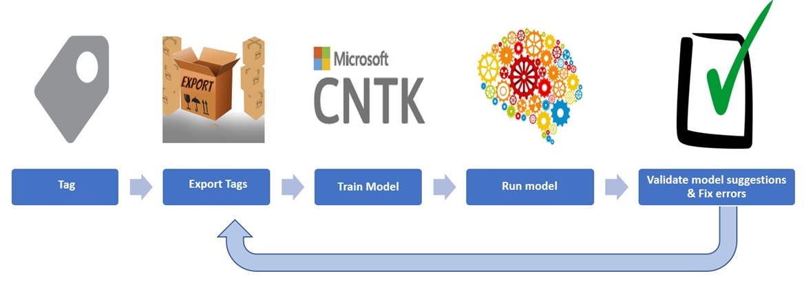
Visual Object Tagging Tool and Microsoft Cognitive Toolkit
The Visual Object Tagging Tool (VoTT) features a great bunch functionalities to kickstart your FAST-RCNN modelling using Microsoft Cognitive Toolkit (used to be called CNTK). It offers an end-to-end solution from tagging your data till deep learning model validation. After loading a bunch of images in VoTT you tag them and the tool will let you export the images in a format ready for your Microsoft Cognitive Toolkit experiment.
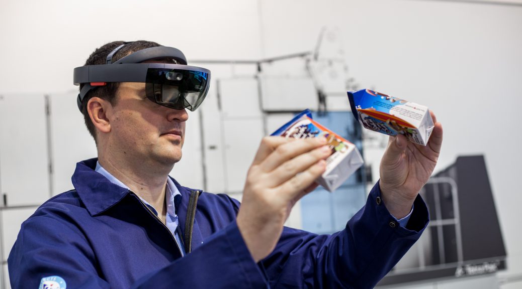
Digital transformation is driving changes in behaviour and business models globally. I’ve had the pleasure to work with Tetra Pak Services and to see first hand how data science and connected devices are shaping our future.
In the video below you see a demo (from Hannover Messe 2017) on how our solution looks like.